numpy cnn
A Convolutional Neural Network implemented in NumPy with modular layers.
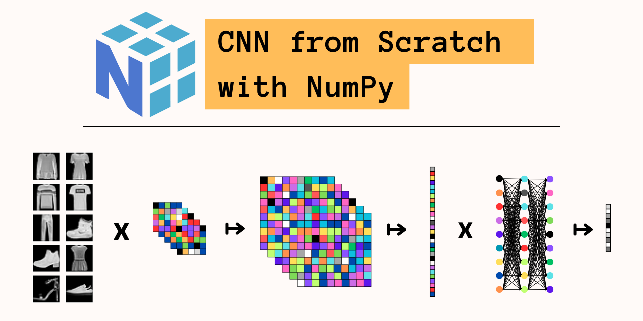
Neural network implementations are more easily accessible now than ever before, abstracting away complexities like gradients, activation layers, and training algorithms. Building neural networks layer by layer from scratch helped me develop a deeper understanding of the structural capabilities and shortcomings of these models. In this project, I implement modular layers for a scalable Convolutional Neural Network using numpy and train it on the Fashion MNIST dataset to perform a simple classification task.
My implementation is both flexible, with variable input, output, kernel, pool sizes, and modular, with separately implemented layers that can be arbitrarily stacked. I achieve an accuracy comparable to a TensorFlow model using the same structure (NumPy Accuracy = 0.891 vs Keras Accuracy = 0.887), albeit with much slower runtime.
This writeup goes in much more detail, but code for this project can be found here.
Table of Contents
- Why Convolutional Neural Networks?
- Fashion MNIST
- The Convolutional Layer
- ReLU Activation
- The Pooling Layer
- The Feedforward Layer
- The Output Layer
- Architecture
- Benchmark
- Sources
Why Convolutional Neural Networks?
Neural networks are made up of three layers: the input, hidden, and output layers. The input layer takes some data (text, images, stock prices, etc.) and processes it for the hidden layer. The hidden layer is where the magic happens: weights and activation fucntions are consecutively applied to the data to extract features necessary to the task at hand. Depending on the task, all kinds of structural complexities can be added to the hidden layer to improve model performance. Finally, these features are passed to the output layer which also uses weights and an activation function to return the desired output. For image classification, this will be a vector whose values represent to the probability that the input image belongs to each class.
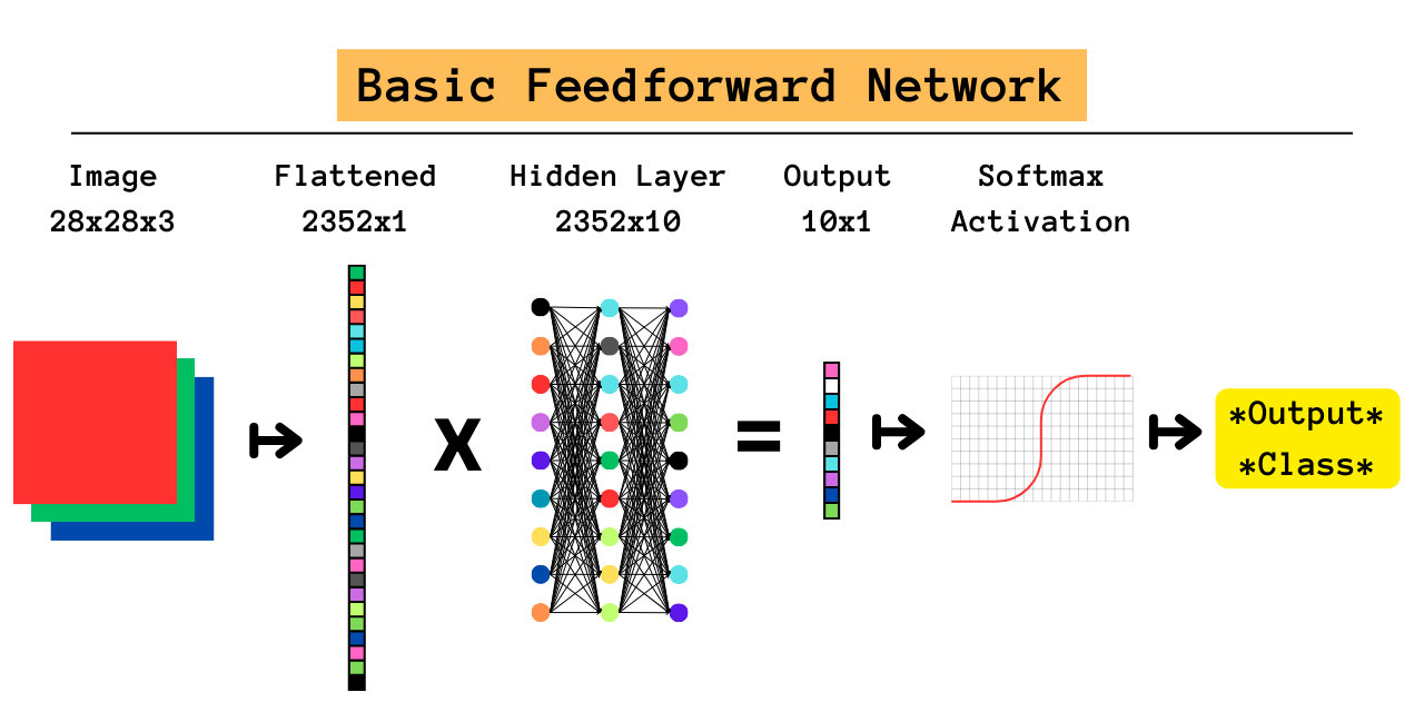
The Feedforward Network (FFN) is a foundational neural network that perfectly illustrates this concept. The network takes a 1-dimensional vector as input, in this case the pixels of an image, and passes it through a number of hidden layers each comprised of a weight matrix and an activation function. The FNN is a naive approach, meaning that almost no assumptions are made about the input data. Since all input data is flattened into a 1-dimensional vector for the network, the weight matrices do all of the heavy lifting. As you can imagine, FNN’s perform poorly on complex tasks and are far outclassed by other models. The reason for this touches on a fundamental concept in model design: gains in predictive power rely on making stronger assumptions about the data and incorporating them into the architecture of the model. Doing so reduces the search space, which removes predictions we know are impossible and improves training efficiency.
Enter the Convolutional Neural Network (CNN), which makes two core assumptions:
- Features can be captured by looking at regions of neighboring pixels;
- Not all pixels are necessary for image classification.
The CNN encodes the first assumption through convolution, which involves sliding a kernel across the input matrix to capture important features. After training, the weights of the kernels highlight parts of the image pertinent to the classification task by combining information within regions of the input matrix. If neighboring pixels within a region indeed contain useful information, the kernels will convert them to better features for classification. The second assumption is encoded through pooling, which systematically reduces matrix size and preserves only the most significant element in each region. The resulting matrix is then passed to a feedforward layer which can be simply a softmax classification layer or even an entire FNN.
Let’s compare these two models classifying a 28x28 pixel RGB image. The FNN converts it into a 28*28*3 = 2352x1 array, so the network cannot infer that the first three elements represent the same pixel or that the next three elements represent a neighboring pixel. As we will see, a simple CNN will produce a 14x14x6 matrix that much better represents the features of the input image; flattening to a 1176x1 array presents the output layer with half as many inputs containing much more significant information.
The Fashion MNIST Dataset
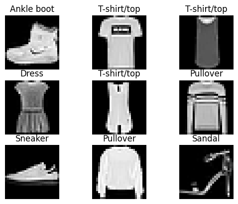
The Fashion MNIST dataset was modeled on the original MNIST database of handwritten digits to provide a more challenging image classification task. While Fashion MNIST is also a set of 70k (60k train and 10k test) black and white 28x28 pixel images, the classes are much more abstract than the original MNIST. Each image is an article of clothing belonging to one of 10 classes: “T-shirt/top”, “Trouser”, “Pullover”, “Dress”, “Coat”, “Sandal”, “Shirt”, “Sneaker”, “Bag”, and “Ankle boot”:
The Convolutional Layer
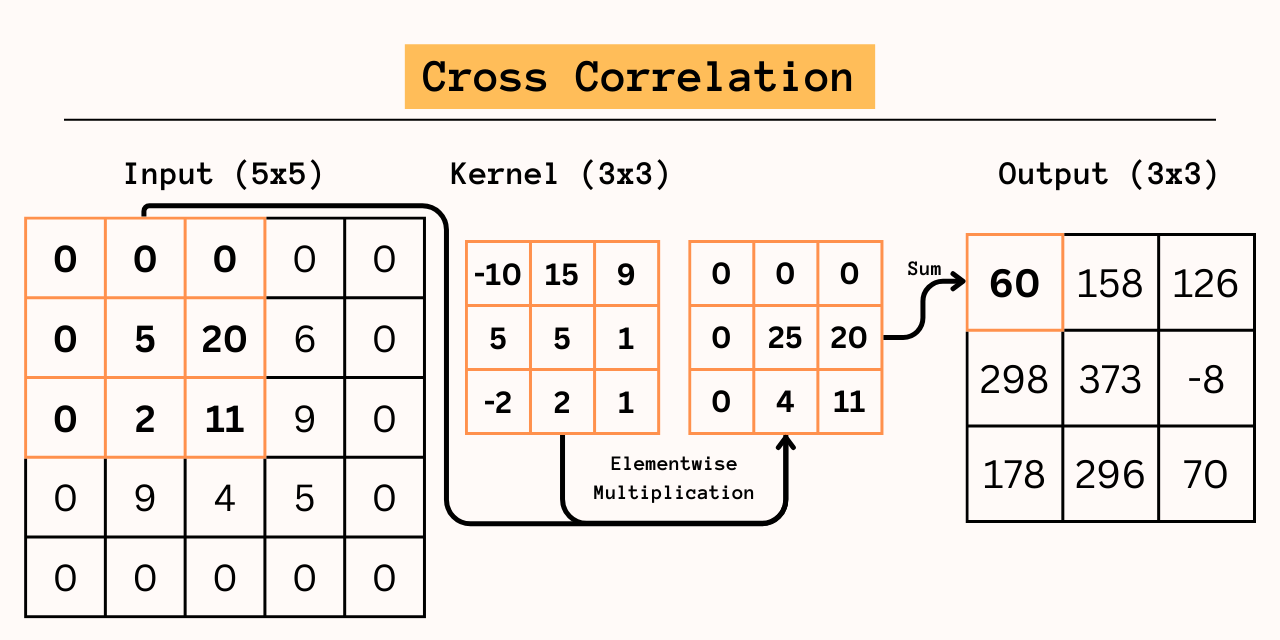
The core of the CNN is convlution: square kernels with odd-numbered length are multiplied elementwise on each region in the image and summed up. Strictly speaking this is cross-correlation; in convlution the kernel has to be rotated by 180°, as seen below. The kernel is iterated across the image in strides and outputs are positionally combined to form a 2D matrix.
1
2
3
4
5
6
7
8
9
10
11
12
13
14
15
16
17
18
 class ConvLayer:
    def __init__(self, input_shape, kernel_size=5, num_kernels=6, padding=0):
        # Get input dimensions
        input_depth, input_height, input_width = input_shape
        self.d = input_depth
        self.h = input_height + kernel_size - 1
        self.w = input_width + kernel_size - 1
        self.input_shape = input_shape
        # Initialize kernels and bias
        self.padding = padding
        self.num_kernels = num_kernels
        self.kernel_size = kernel_size
        self.pad_size = kernel_size // 2
        self.kernel_shape = (self.num_kernels, self.d, self.kernel_size, self.kernel_size)
        self.bias_shape = (self.num_kernels, self.h - self.kernel_size + 1, self.w - self.kernel_size + 1)
        # Dividing mimics Xavier Initialization and reduces variance
        self.kernels = np.random.randn(*self.kernel_shape) / (self.kernel_size * self.kernel_size)
        self.bias = np.random.randn(*self.bias_shape) / (self.h * self.w)
Notice that the resulting array will be smaller than the original image. In order to produce arrays of equal size, this implementation pads the array with borders of zeroes (border size 2 for the 5x5 kernel), called full convolution as opposed to valid convlution. In this implementation, kernel weights and biases are customizeable by size and number.
Forward
1
2
3
4
5
6
7
8
9
10
11
12
13
14
15
16
17
18
19
20
21
 class ConvLayer:
    #...
    def iter_regions(self, image):
        """
        Generates all possible (kernel_size x kernel_size) image regions (prepadded)
        """
        for i in range(self.h - self.kernel_size + 1):
            for j in range(self.w - self.kernel_size + 1):
                im_region = image[:, i:(i + self.kernel_size), j:(j + self.kernel_size)]
                yield im_region, i, j

    def forward(self, input):
        """
        Pad input, get regions, and perform full cross correlation with kernels
        """
        padded = np.pad(input, ((0,0), (self.pad_size, self.pad_size), (self.pad_size, self.pad_size)), mode="constant", constant_values=self.padding)
        self.prev_input = padded # Save for backpropagation
        self.output = np.copy(self.bias)
        for im_region, i, j in self.iter_regions(padded):
            self.output[:, i, j] += np.sum(im_region * self.kernels, axis=(1, 2, 3))
        return self.output
The forward() function is straightforward:
- Pad the input matrix according to kernel size;
- Using the
iter_regions()method, get all regions that need to be cross-correlated with the kernel; - Perform the cross correlation by multiplying elementwise (numpy’s multiply function does this by default) and then sum up elements on all axes.
Since we generally work with more than one kernel and input matrices are often 3D, we can stack kernels into a 4D matrix that can be easily multiplied with the 3D input array. The regions will be multiplied along the first dimension of the kernel array and summed up along the other three dimensions which will generate a 1D vector representing the output of each kernel on the region.
Backpropagation
1
2
3
4
5
6
7
8
9
10
11
12
13
14
15
16
17
18
19
20
21
22
 class ConvLayer:
    #...
    def backprop(self, d_L_d_out, learn_rate):
        """
        Update kernels and bias, and return input gradient
        """
        # Cross correlation for kernel gradient
        d_L_d_kernels = np.zeros(self.kernels.shape)
        for im_region, i, j in self.iter_regions(self.prev_input):
            for f in range(self.num_kernels):
                d_L_d_kernels[f] += d_L_d_out[f, i, j] * im_region
        # Full convolution for input gradient
        d_L_d_input = np.zeros(self.input_shape)
        pad_out = np.pad(d_L_d_out, ((0,0), (self.pad_size, self.pad_size), (self.pad_size, self.pad_size)), mode="constant", constant_values=0)
        conv_kernels = np.rot90(np.moveaxis(self.kernels, 0, 1), 2, axes=(2, 3))
        for im_region2, i, j in self.iter_regions(pad_out):
            for d in range(self.d):
                d_L_d_input[d, i, j] += np.sum(im_region2 * conv_kernels[d])
        # Adjust by learn rate
        self.bias -= learn_rate * d_L_d_out
        self.kernels -= learn_rate * d_L_d_kernels
        return d_L_d_input
The backpropagation for the convolutional layer is much more complicated, especially since an input gradient must also be calculated to backpropagate to lower layers. Terminology for backpropagation may be tricky here: the input gradient is the gradient of the input matrix during the forward phase. For the first layer, that matrix represents the input image. The output gradient is the input to the backprop() function, which for the output layer is the initial gradient calculated with the gold standard label. The bias gradient is easiest to resolve: since it is the base of the output, it should simply be adjusted by the output gradient.
To understand backpropagating the kernel weights, consider that each kernel is iterated across the input matrix and apply to all regions equally, which means that each region of the gradient should have some effect on the kernel. The kernel gradient is therefore the sum of the product between the output gradient and the previous input matrix for each region of kernel size.
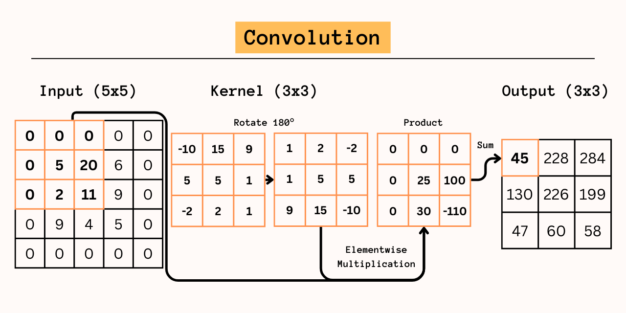
The input gradient is where we encounter convolution. Without going into too much mathematical detail, consider that each input element has a different and unequal effect on the output: corner elements will only contribute to the one corner element in the output whereas edges and central elements will contribute to multiple output elements. This same pattern occurs when calculating the derivative with respect to the input elements, since output elements that were not calculated with the input element will have a derivative of 0 with respect to that input element. The key difference is that each output element is affected by the opposite kernel element, which means that the kernel must be rotated 180° (precisely as in convolution) in order to calculate the gradient for the input element. In order to produce this pattern, a full convolution must be used, even for models that use valid cross-correlation in the forward() portion.
ReLU Activation
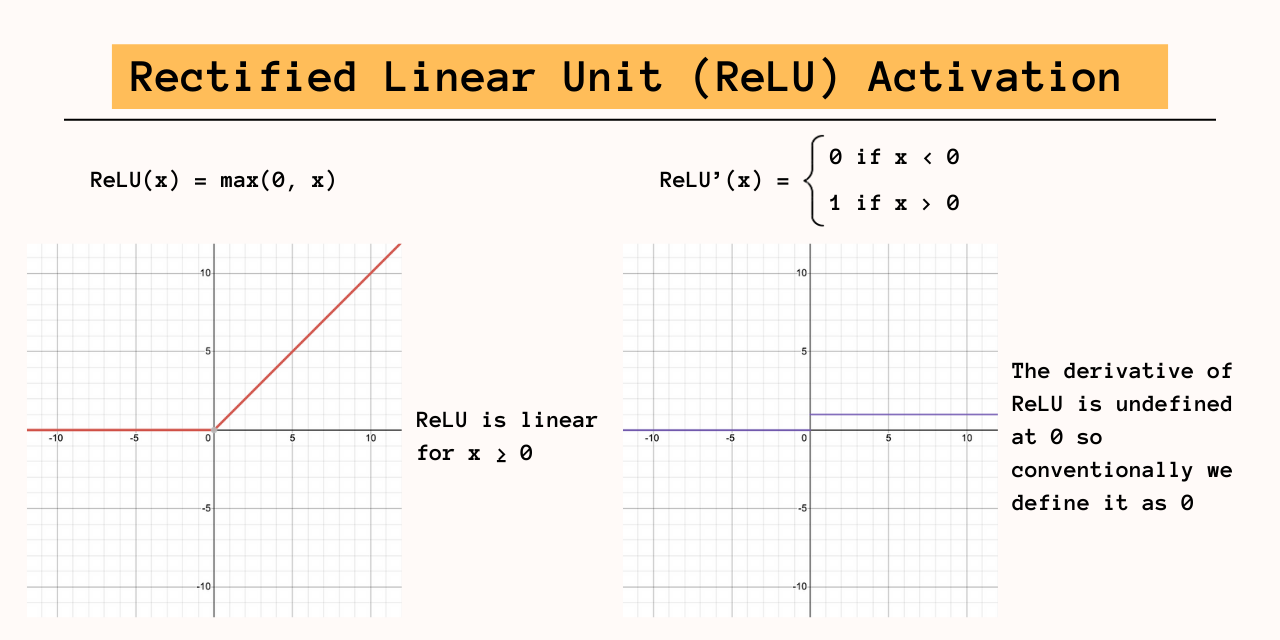
At the core of the neural network is the activation function, which is applied to the outputs of the previous layer to introduce nonlinearity. Without activation, stacked layers remain linear and have the same predictive power as a single layer. The downside to the nonlinear function occurs in backpropagation, where certain outputs can result in disappearing gradients breaking the training loop. For this reason, many models prefer using ReLU as the activation function for non-terminal layers. ReLU behaves linearly for inputs greater than 0 which means its derivative is 1, preventing disappearing gradients while maintaining nonlinearity. The derivative of ReLU is undefined at 0 conventionally we set it to 0.
1
2
3
4
5
6
7
8
9
10
11
12
13
 class ReLU:
    """
    Simple ReLU activation function
    """
    def __init__(self):
        pass

    def forward(self, input):
        self.prev_output = np.maximum(0, input)
        return self.prev_output

    def backprop(self, d_L_d_out):
        return d_L_d_out * np.int64(self.prev_output > 0)
As seen in the code, the ReLU class implemented here is easy to use. Once we run forward() the function will take the shape of the previous output. The backprop() function is also straightforward, simply passing all outputs that were not zeroed out by ReLU and multiplying by the gradient.
The Pooling Layer
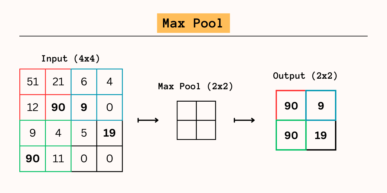
We’ve seen that kernels in the convolutional layer capture information from neighboring pixels, which means that many elements in the output array contain redundant information. While this is hardly an issue for the 28x28 Fashion MNIST images, computation can quickly get out of hand for multilayer networks processing images with thousands of pixels. Pooling presents a simple solution: run another square array across the output matrix and at each stride keep only the max, min, or mean value. Pooling only makes sense because of our second assumption that neighboring pixels contain redundant information, which is true of the convolutional layer output.
1
2
3
4
5
6
7
8
9
10
11
12
13
14
15
16
17
18
19
20
21
22
23
24
25
26
27
28
29
30
31
32
33
34
35
36
37
38
39
40
41
 class MaxPool:
    def __init__(self, pool_size=2):
        self.size = pool_size

    def iter_regions(self, image):
        """
        Same as Conv layer, but with stride of pool_size
        """
        _, h, w = image.shape
        new_h = h // self.size
        new_w = w // self.size
        for i in range(new_h):
            for j in range(new_w):
                im_region = image[:, (i * self.size):(i * self.size + self.size), (j * self.size):(j * self.size + self.size)]
                yield im_region, i, j

    def forward(self, input):
        """
        Gets max value in each region
        """
        self.prev_input = input
        num_kernels, h, w = input.shape
        output = np.zeros((num_kernels, h // self.size, w // self.size))
        for im_region, i, j in self.iter_regions(input):
            output[:, i, j] = np.amax(im_region, axis=(1, 2))
        return output

    def backprop(self, d_L_d_out):
        """
        Backpropagates gradient to input
        """
        d_L_d_input = np.zeros(self.prev_input.shape)
        for im_region, i, j in self.iter_regions(self.prev_input):
            f, h, w = im_region.shape
            amax = np.amax(im_region, axis=(1, 2))
            for i2 in range(h):
                for j2 in range(w):
                    for f2 in range(f):
                        if im_region[f2, i2, j2] == amax[f2]:
                            d_L_d_input[f2, i * self.size + i2, j * self.size + j2] = d_L_d_out[f2, i, j]
        return d_L_d_input
This implementation uses a 2x2 max pool, but any value will evenly reduce the size of the output while keeping the most important information. The size of the pool should be balanced with the size of the kernel in the convolutional layer; At minimum, each pooling layer reduces the size of the input by a factor of 4. Since no weights are learned, the forward() and backprop() is deterministic. In the forward pass, the input array is reduced by the method described. In the backpropagation portion, we simply place the gradient values in their respective positions in the input matrix and set all other values to zero.
The Feedforward Layer
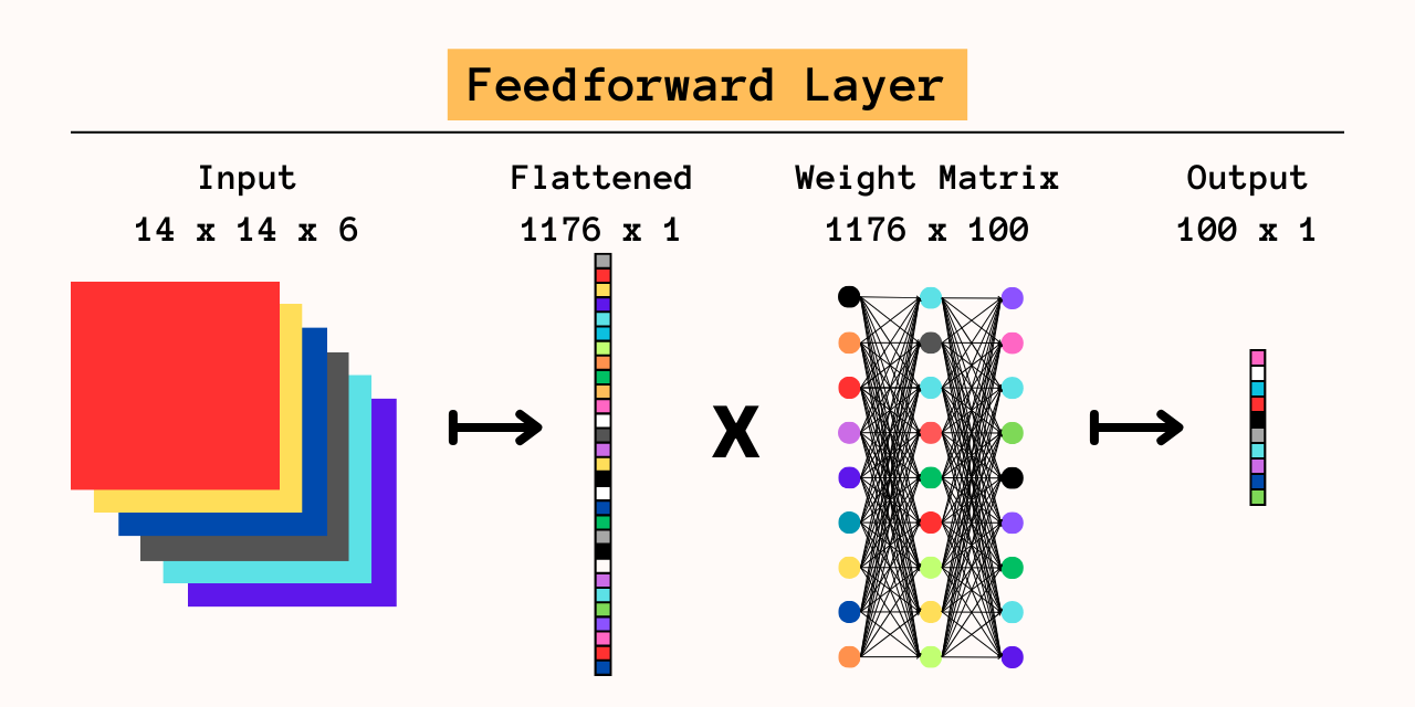
We now have a working system for extracting features from input images using convolution, which leaves only the classification step left. For smaller models, a single softmax classification layer as seen below may be sufficient, but generally a full feedforward network is used for prediction. The feedfoward layer collapses the input matrix into a 1-dimensional array, with each element of the array representing a separate feature for the feedforward network.
1
2
3
4
5
6
7
8
9
10
11
12
13
14
15
16
17
18
19
20
21
22
23
24
25
26
 class FeedForward:
    def __init__(self, input_size, output_size):
        self.weights = np.random.randn(input_size, output_size) / input_size
        self.bias = np.random.randn(output_size) / output_size

    def forward(self, input):
        """
        Multiply by weights and add bias
        """
        self.prev_input_shape = input.shape
        input = input.flatten()
        self.prev_input = input
        self.output = np.dot(input, self.weights) + self.bias
        return self.output

    def backprop(self, d_L_d_out, learn_rate):
        """
        Update weights and bias, and return input gradient
        """
        d_out_d_weights = self.prev_input
        d_out_d_input = self.weights
        d_L_d_weights = d_out_d_weights[np.newaxis].T @ d_L_d_out[np.newaxis]
        d_L_d_input = d_out_d_input @ d_L_d_out
        self.weights -= learn_rate * d_L_d_weights
        self.bias -= learn_rate * d_L_d_out
        return d_L_d_input.reshape(self.prev_input_shape)
Multiplying with a weight matrix returns an array of the desired size, and an activation function is used to achieve nonlinearity. The backprop() function is fairly straightforward: the output gradient is multiplied by the previous input to get the gradients for the weights, the output gradient is the bias gradient, and the input gradient is the product of the weights and the output gradient.
The Output Layer
The output layer is the same as in other networks performing classification tasks: a number of features are passed in, multiplied by a weight matrix to get the correct number of outputs and run through a softmax function (or sigmoid function for binary classification) to get an output array representing the probability for each class. The only differences between the output and feedforward layers are in the activation function and backpropagation.
1
2
3
4
5
6
7
8
9
10
11
12
13
14
15
16
17
18
19
20
21
22
23
24
25
26
27
28
29
30
31
32
33
34
35
36
37
38
39
40
41
42
43
44
45
 class Softmax:
    def __init__(self, input_len, nodes):
        self.weights = np.random.randn(input_len, nodes) / input_len
        self.bias = np.random.randn(nodes) / nodes

    def forward(self, input):
        """
        Flatten input, matrix multiply with weights, add bias, and get softmax
        """
        # Forward pass
        totals = np.dot(input, self.weights) + self.bias
        exp = np.exp(totals)
        # Saving forward pass for backpropagation
        self.prev_input_shape = input.shape
        self.prev_input = input
        self.prev_totals = totals
        return exp / np.sum(exp, axis=0)

    def backprop(self, d_L_d_out, learn_rate):
        """
        Softmax backprop for output layer
        """
        for i, gradient in enumerate(d_L_d_out):
            # Only the gradient at the correct class is nonzero
            if gradient == 0:
                continue
            # e^totals
            t_exp = np.exp(self.prev_totals)
            S = np.sum(t_exp)
            # Gradients at i against totals
            d_out_d_t = -t_exp[i] * t_exp / (S ** 2)
            d_out_d_t[i] = t_exp[i] * (S - t_exp[i]) / (S ** 2)
            # Gradients of totals against weights/bias/input
            d_t_d_w = self.prev_input
            d_t_d_b = 1
            d_t_d_inputs = self.weights
            # Gradients of loss against totals
            d_L_d_t = gradient * d_out_d_t
            d_L_d_w = d_t_d_w[np.newaxis].T @ d_L_d_t[np.newaxis]
            d_L_d_b = d_L_d_t * d_t_d_b
            d_L_d_inputs = d_t_d_inputs @ d_L_d_t
            # Update weights and bias
            self.weights -= learn_rate * d_L_d_w
            self.bias -= learn_rate * d_L_d_b
            return d_L_d_inputs.reshape(self.prev_input_shape)
Generally, the output layer always uses a sigmoid or softmax activation function since these functions convert unbounded numbers into probabilities. However, since these functions are prone to vanishing gradient issues, they are almost never used for intermediary layers. For convenience, I implement the softmax function directly into the output layer class, although they can be separated as with the ReLU function. The backprop() function for the output layer needs to take into account the fact that the gradient is only nonzero for the gold standard class but is otherwise the same as in the feedforward layer.
Model Architecture
All the layers are done, let’s put them together!

As you can see, this is the simplest architecture that uses all of the layers of the CNN. At the same time, we can add as many convolutional layer -> convolutional layer -> pooling layer stacks as we want for arbitrary depth. Depending on the size of the model, we can also have multiple feedforward layers to increase the predictive power of the classification portion of the network. Empirically, lower convolutional layers in deep networks learn to identify basic shapes such as edges whereas higher layers learn more complex features such as body parts.
1
2
3
4
5
6
7
8
9
10
11
12
13
14
15
16
17
18
19
20
21
22
23
24
25
26
27
28
29
30
31
32
33
34
35
36
37
38
39
40
41
42
43
44
45
46
47
48
49
50
51
52
53
54
55
56
57
58
59
60
61
62
63
64
65
66
67
68
69
70
71
72
73
74
75
76
77
78
79
80
81
82
83
84
85
86
87
88
89
90
91
92
93
94
95
96
97
98
99
100
101
102
103
104
105
106
107
108
109
110
111
112
113
114
115
116
117
118
119
120
121
122
123
124
125
126
127
128
129
130
131
132
133
134
 class SimpleCNN:
    """
    Simple CNN using the layers built above.
    Structure:
    Input -> Conv -> ReLU -> Conv -> ReLU -> MaxPool -> FeedForward -> ReLU -> Softmax
    """
    def __init__(self, ConvLayer_1, ReLU_1, ConvLayer_2, ReLU_2, MaxPool, FeedForward, ReLU_3, Output):
        self.ConvLayer_1 = ConvLayer_1
        self.ReLU_1 = ReLU_1
        self.ConvLayer_2 = ConvLayer_2
        self.ReLU_2 = ReLU_2
        self.MaxPool = MaxPool
        self.FeedForward = FeedForward
        self.ReLU_3 = ReLU_3
        self.OutputLayer = Output

    def preprocess(self, data):
        """
        Data generally needs to be reshaped for our purposes
        """
        if len(data.shape) == 3:
            data = data[:, np.newaxis, :, :]
        elif len(data.shape) == 4 and data.shape[3] == 3:
            data = np.moveaxis(data, -1, 1)
        return data

    def forward(self, image):
        """
        Forward pass through network, transform image from [0, 255] to [-0.5, 0.5] as standard practice
        """
        input = (image / 255) - 0.5
        out = self.ConvLayer_1.forward(input)
        out = self.ReLU_1.forward(out)
        out = self.ConvLayer_2.forward(out)
        out = self.ReLU_2.forward(out)
        out = self.MaxPool.forward(out)
        out = self.FeedForward.forward(out)
        out = self.ReLU_3.forward(out)
        out = self.OutputLayer.forward(out)
        return out

    def backprop(self, gradient, learn_rate):
        """
        Backpropagation through network
        """
        d_L_d_out = self.OutputLayer.backprop(gradient, learn_rate)
        d_L_d_out = self.ReLU_3.backprop(d_L_d_out)
        d_L_d_out = self.FeedForward.backprop(d_L_d_out, learn_rate)
        d_L_d_out = self.MaxPool.backprop(d_L_d_out)
        d_L_d_out = self.ReLU_2.backprop(d_L_d_out)
        d_L_d_out = self.ConvLayer_2.backprop(d_L_d_out, learn_rate)
        d_L_d_out = self.ReLU_1.backprop(d_L_d_out)
        d_L_d_out = self.ConvLayer_1.backprop(d_L_d_out, learn_rate)
        return d_L_d_out

    def avg_f1_score(self, predicted_labels, true_labels, classes):
        """
        Calculate the f1-score for each class and return the average of it
        F1 score is the harmonic mean of precision and recall
        Precision is True Positives / All Positives Predictions
        Recall is True Positives / All Positive Labelsß
        """
        f1_scores = []
        for c in classes:
            pred_class = np.array([pred == c for pred in predicted_labels])
            true_class = np.array([lab == c for lab in true_labels])
            precision = (t_sum(logical_and(pred_class, true_class)) / t_sum(pred_class)) if t_sum(pred_class) else 0
            recall = t_sum(logical_and(pred_class, true_class)) / t_sum(true_class)if t_sum(true_class) else 0
            f1_scores.append(2 * (precision * recall) / (precision + recall)) if precision and recall else 0
        return np.mean(f1_scores)

    def predict(self, dataset, true_labels, classes):
        """
        Predict labels for dataset and return f1-score
        """
        preds = []
        acc = 0
        for im, lab in zip(dataset, true_labels):
            preds.append(np.argmax(self.forward(im)))
            acc += (preds[-1] == lab)
        preds = np.array(preds)
        accuracy = acc / len(preds)
        f1 = self.avg_f1_score(preds, true_labels, classes)
        return accuracy, f1

    def train(
        self,
        trainset,
        trainlabels,
        devset,
        devlabels,
        classes=[0, 1, 2, 3, 4, 5, 6, 7, 8, 9],
        epochs=3,
        learn_rate=0.005
    ):
        """
        Training loop for network
        """
        # Preprocess & generate permutation to shuffle data
        trainset = self.preprocess(trainset)
        devset = self.preprocess(devset)
        permutation = np.random.permutation(len(trainset))
        train_data = trainset[permutation]
        train_labels = trainlabels[permutation]
        # Training loop
        print("Training...")
        for epoch in range(epochs):
            losses = []
            for image, label in tqdm(list(zip(train_data, train_labels))):
                # Forward pass
                out = self.forward(image)
                # Calculate loss and gradient
                loss = -np.log(out[label])
                losses.append(loss)
                gradient = np.zeros(10)
                gradient[label] = -1 / out[label]
                # Backpropagation
                self.backprop(gradient, learn_rate)
            print(f"Epoch {epoch + 1}, loss: {np.mean(losses):.3f}")
            print("Evaluating dev...")
            acc, f1 = self.predict(devset, devlabels, classes)
            print(f"Dev Accuracy: {acc:.3f}, Dev F1 Score: {f1:.3f}")

model = SimpleCNN(
        ConvLayer(input_shape=(1, 28, 28), kernel_size=5, num_kernels=6, padding=0),
        ReLU(),
        ConvLayer(input_shape=(6, 28, 28), kernel_size=5, num_kernels=6, padding=0),
        ReLU(),
        MaxPool(),
        FeedForward(6 * 14 * 14, 100),
        ReLU(),
        Softmax(100, 10)
)
model.train(trainset, trainlabels, testset, testlabels, epochs=3, learn_rate=0.005)
The model class and training loop are to implement since the forward() and backprop() functions have been properly implemented. Before training, I use np.random.permutation() to randomize the training set in case the original initialization is suboptimal. Although the dataset is in black and white, the layers are built to handle 3D inputs like RGB images. As a result, a preprocess function is needed to handle the 2D inputs in the Fashion MNIST dataset and to adjust the channel dimension for RGB images. RGB images are usually processed as height x width x channel matrices, however, for convenient matrix multiplication the channel matrix needs to be moved up to channel x height x width. Using this implementation, the multiplication done in the convolutional layer can be done natively in NumPy instead of utilizing additional for loops.
Benchmarking with Keras
1
2
3
4
5
6
7
8
9
10
11
12
13
14
15
16
17
18
19
20
21
22
23
24
25
26
27
28
29
 from keras.models import Sequential
from keras.layers import Conv2D, MaxPooling2D, Dense, Flatten
from keras.utils import to_categorical
from keras.optimizers.legacy import SGD

train_images = (trainset / 255) - 0.5
test_images = (testset / 255) - 0.5

train_images = np.expand_dims(train_images, axis=3)
test_images = np.expand_dims(test_images, axis=3)

model = Sequential([
  Conv2D(6, 5, padding="same", input_shape=(28, 28, 1), use_bias=True, activation='relu'),
  Conv2D(6, 5, padding="same", input_shape=(28, 28, 6), use_bias=True, activation='relu'),
  MaxPooling2D(pool_size=2),
  Flatten(),
  Dense(100, activation='relu'),
  Dense(10, activation='softmax'),
])

model.compile(SGD(learning_rate=.005), loss='categorical_crossentropy', metrics=['accuracy'])

model.fit(
  train_images,
  to_categorical(trainlabels),
  batch_size=1,
  epochs=3,
  validation_data=(test_images, to_categorical(testlabels)),
)
Here’s a Keras model implemented using the exact same architecture as above to benchmark performance. Since Keras is an optimized library with widespread adoption, running time is predictably orders of magnitude faster than my implementation.
Results
NumPy model: F1 = 0.890, Accuracy = 0.891
Keras model: Accuracy = 0.887
My model surprisingly outperforms the Keras model by a little, which suggests that the underlying mechanisms in both implementations are the same. I achieve an F1 = 0.890 training 3 epochs on the entire dataset, taking roughly half an hour per epoch. While these results are significantly lower than the state of the art F1 = 0.97, theoretically a deeper network using the same layers could potentially achieve comparable results with enough computation.